Benchmarking the Performance of Automated Liquidity Vault Strategies

This is the latest installment in a series of posts by 0xfbifemboy about the design, performance, and utility of concentrated liquidity and AMMs.
Introduction
Originally, with fully ambient, constant-product AMMs such as Uniswap V2, liquidity providers (LPs) only had one choice to make in any given liquidity pool: what percentage of their portfolio to allocate to supplying ambient liquidity, from 0% to 100%. That is to say, the only parameters they could tune were (1) whether or not they were in the pool at all and (2) if so, then how much money they should put in.
This situation changed dramatically with the release of Uniswap V3, which introduced a notion of concentrated or range-bound liquidity. By specifying a lower and upper price bound for supplied liquidity, V3 LPs were able to reap higher proportions of trading fees relative to V2 LPs with the same amount of starting capital; however, these positions then expose the user to more impermanent loss, and if the pool price moves outside of a given liquidity position’s range, zero fees are accrued by that position. This extended, in principle, the ability of a liquidity provider to implement a sophisticated market-making strategy through active management of Uniswap liquidity positions.
With the popularity of yield farming throughout 2021, this naturally motivated the development of managed liquidity positions, or vaults, where users would deposit tokens and a protocol would implement some sort of active liquidity management strategy on Uniswap V3 to deliver yield to the user. Many such protocols spun up in the second half of 2021 (immediately following the release of Uniswap V3), such as Gelato Network, Charm Finance, etc. Naturally, these vaults appealed to users who wanted to capture the theoretically very high yields of a sophisticated market making strategy on Uniswap V3 without having to actually make those markets themselves.
The problems faced by liquidity vaults are not specific to liquidity vaults alone. When a new DEX is starting up or a new token is launching, it is of course highly desirable to be able to supply cheap liquidity. To be precise, a yield farmer who deposits into an actively managed vault seeks to maximize total return, whereas the developer of a new token seeks to maximize total return per unit of active liquidity supplied. These are highly interrelated concepts and the same framework can be used to understand both simultaneously.
However, despite the proliferation of these vaults and the clear utility of understanding effective active management strategies, there has been no systematic comparison of active strategy performance to date. Is it possible to analyze vaults’ performance empirically, to see if they live up to their claims? If not, is it possible to backtest the strategies that protocols describe themselves as using? What should our expectations be about how hard it is to design a profitable vault strategy? These questions clearly highlight a gap in the extensive AMM discourse so far. In this post, we present an initial series of simple backtest analyses which begin to shed light on the myriad challenges of active liquidity management.
Overview of existing vault strategies
In general, it is challenging to analyze vault performance. Different protocols use bespoke contracts which need to be individually analyzed (and their event logs may not emit all the necessary information); vaults often do not hold Uniswap V3 NFTs, so linking together metadata across contract calls is laborious and tricky; centrally maintained strategies are not necessarily implemented in a consistent way throughout the life of the vault; and so on and so forth.
Instead of tediously parsing on-chain data from multiple complex protocols, we aimed at a simpler approach:
- Figure out what protocols say they are doing
- Backtest their strategies
This approach benefits from consistency of implementation and analysis. Additionally, as we will soon see, vault protocols more or less describe themselves as implementing very similar strategies, allowing us to obtain straightforward results with little effort that generalize across a wide range of realistic scenarios.
First off, we have to begin by understanding what strategies vault protocols claim to use. We will simply quote from them one at a time.
On the other hand, active G-UNI’s will always target providing liquidity as efficiently as possible around e.g. 5%-10% above or below the current trading price, but still in a completely trustless and automated fashion. This is achieved by having Gelato bots monitor the average price and every 30 minutes will decide to rebalance only if the average trading price is outside the current bounds of the position. If that is the case, rebalancing happens, and the position is withdrawn and redeposited with the proper adjustment to the new trading price.
Consider UniV3 ETH/USDC 0.05% pool and assume we’d like to put our liquidity into the [1000, 2000] price range (we refer to it as the Domain price range). How can we do better than just providing it directly into the pool?
The trick is to put only a tiny portion of liquidity into a really narrow price range earning the same fees as direct providing. As soon as the price risks going out of the narrow range, rebalance the interval to cover the price safely.
According to Gamma, their strategies are based on backtesting of past prices and other time-series forecasting methods such as Bollinger bands, empirical probabilities, and machine learning algorithms. Currently, Gamma is employing an Autoregressive strategy based on mean reversion. In essence, a statistical model is used to dynamically set the center and width of the liquidity ranges depending on recent market behavior. By doing so, it uses the concept of mean reversion to predict where the price will go, further increasing the time spent in-range and mitigating impermanent loss.
The strategy always maintains two active range orders:
-Base order centered around current price X, in the range [X-B, X+B]. If B is lower, it will earn a higher yield from trading fees.
-Rebalancing order just above or below the current price. It will be in the range [X-R, X], or [X, X+R], depending on which token it holds more of after the base order was placed. This order helps the strategy rebalance and get closer to 50/50 to reduce inventory risk.
There are possibly more liquidity vault protocols out there; that being said, there has been a great deal of renaming, merging, and pivoting to or away from vault management in this space, and we feel that these four quoted passages are fairly representative.
In general, the idea is to create a range position centered at the current price and to rebalance it after the price deviates sufficiently, creating a new liquidity position centered on the now-current price. This is the approach taken by Gelato and Mellow. It can be extended in many ways; for example, Mellow uses a second range order to “assist” with the rebalancing process, while Gamma uses statistical estimates of mean reversion in order to appropriately size liquidity range positions. We will therefore begin by examining the simplest possible case, that of a single range position that recenters itself whenever the price is out of range, and subsequently consider extensions to this model.
Backtesting a simple rebalancing strategy
We will analyze these strategies primarily from the perspective of a DEX or a protocol wishing to seed initial token liquidity at the lowest cost possible, rather than from a “retrospective analysis of vault performance” point of view. That is to say, these results will be, by design, more useful to developers of new protocols rather than yield farmers seeking to optimize yields. Therefore, we will only be indirectly looking at the performance of liquidity vaults, although we feel that our results are still quite informative to would-be yield farmers.
This design choice enables us to make a major simplification: We will take the price of ETH over the last year or so at a 10-minute resolution and assume that there is only arbitrage flow, so that the only swap fees earned by any in-range liquidity position are essentially the minimal fees necessary to bring the pool price from one point to another. This is a very extreme assumption, but it simplifies calculation substantially, reduces variability in the results originating from the (in)activity of other LPs, and still allows us to make relative comparisons between different rebalancing strategies, even if our estimates of the absolute returns are off. Additionally, while this is an odd assumption from the perspective of retrospective analysis of liquidity vaults, it is actually quite a reasonable assumption from our desired perspective of a protocol or DEX wishing to minimize its “cost for liquidity,” because on a new trading platform or in a new pool, we cannot make optimistic assumptions about the quantity of uninformed flow we will receive, and these “worst-case” estimates are actually very relevant!
Additionally, we assume that the simulated liquidity provider starts with an arbitrary fixed amount of capital, in our case $1,000,000 USD. As the rebalancing strategy is implemented and the price of ETH naturally changes, the net portfolio value of the LP’s position may change above or below that initial $1m value. Again keeping in mind our desired perspective, we assume that it is desirable for the liquidity provider to continually “top-up” shortfalls in the position value, so that a somewhat consistent dollar value of liquidity is supplied over time. Additionally, as the price of ETH evolves over time, we keep track of the total IL incurred by the liquidity provider (relative to the starting point of each rebalance); in both a protocol/DEX context and a yield-farming context, sophisticated users are likely to have delta exposure hedged out, so we feel this is the correct primary metric to look at.
Let us first consider the above scenario parameterized by a single variable C > 1 which is the width of a new liquidity position: if the current pool price is p, then a new range position is given by the interval [p/C, p*C]. For example, if C = 1.01 (a very low value), then range positions are created approximately 1% above and below the current price of ETH. If C = 2 and the price of ETH is $1,000, then a range position goes from a lower bound of $500 to an upper bound of $2,000. Note that in Uniswap tick space this corresponds to a constant offset subtracted from or added to the current price tick, and hence accurately corresponds to the notion of a "centered" or "balanced" position. Whenever the price moves outside of the position's active range, the entire position is assumed to be liquidated and recreated at the same width around the new price.
We can learn a surprising amount from this simple example alone! We will initially consider a case of 0 swap fees, so we look purely at the IL that different strategies (corresponding to different values of C) are exposed to. Suppose we run this simulation for C = 1.01, 1.1, 1.5, 2 and plot the ratio of accumulated IL to initial capital:
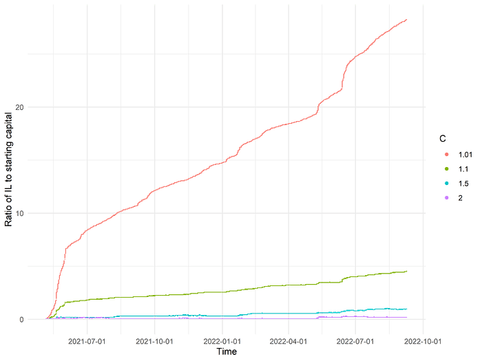
The differences are striking! If we use a position width of 1%, then over the course of about 15 months, our position loses nearly 30 times its initial value in exposure to impermanent loss alone! Recall, of course, that we previously specified that at each rebalance point, the nominal USD value of the liquidity position is topped up back to the initial value of $1 million. (We could have not made this assumption, in which case we would just have seen the ratio of IL to starting capital approach 1 very early on.)
To be precise, for C = 1.01, 1.1, 1.5, 2, the losses in terms of IL to starting capital are, respectively, 25, 4, 0.9, and 0.2 (approximately). Clearly, at this range of parameter values, wider positions subject the liquidity provider to substantially reduced losses. If we look at the number of rebalances in each run—respectively 6048, 151, 8, and 1—we begin to suspect that the frequency of position rebalancing relates to the degree of exposure to IL.
We can gain further insight by looking at the evolution of the IL-to-capital ratio over time for a single run, say, C = 1.5, which has sufficiently few rebalance events that the corresponding graph has visually discernible structure:
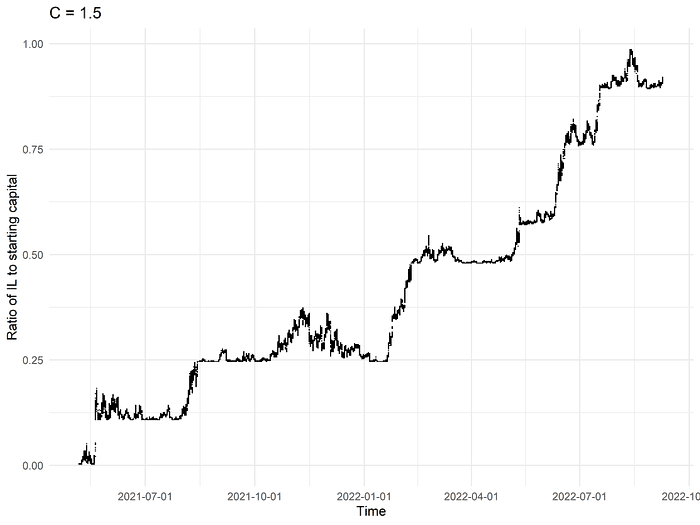
Almost immediately, we notice a very distinct pattern. It appears that the degree of IL exposure tends to plateau for a while before suddenly “jumping up” to a new level, staying there and oscillating for another while, then “jumping up” again, and so on. This makes sense if we consider what it means, mechanically, for the position to rebalance. Suppose that we have a range position from, say, $1,000 to $2,000. As the price of ETH oscillates within this interval, the “unrealized IL” fluctuates, reaching zero at the midpoint of the range position and reaching its maximal values at the endpoints of $1,000 and $2,000. If we insist that the position must rebalance as soon as it goes out of range, we are in effect “locking in” a very large amount of IL.
In the case of C = 1.01, it is easy to see why this strategy performs so poorly. ETH moves more than 1% in either direction multiple times in a day. Effectively, then, what we are doing is continually selling local bottoms and buying local tops over and over again (about once every 2-3 hours!). In this sense, it is unsurprising that the degree of realized IL exposure is so high after a year of this horrible trading strategy!
To analyze these phenomena more systematically, we tested a wider range of values of C. As we might have suspected from the prior discussion, as C increases, the amount of realized IL at the end of the simulation period drops sharply:
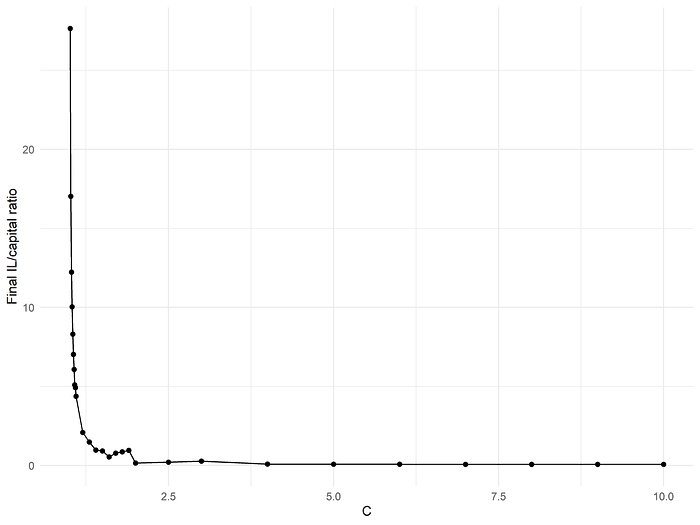
Of course, after C = 4 or so, we are at the point where there are no rebalances whatsoever, and the only remaining "gains" come from diffusing liquidity over a wider and wider range (asymptotically approaching ambient liquidity). If we are a protocol wishing to "seed" token liquidity, what we are really interested in is the cost per unit of active liquidity:
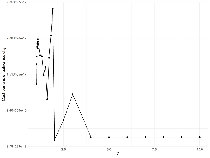
(Note: In the above graph, the cost per unit of active liquidity is normalized by scaling all values upward by a fixed factor. This transformation is arbitrary, and performed solely for readability. Because every dollar of liquidity corresponds to a very large number of liquidity units, the original values are extremely small and hard to interpret. Instead, they have all been multiplied by a fixed factor equal to the number of liquidity units that make up a single dollar of ambient liquidity at the starting price of ETH in this dataset. This is a little unnatural in the current context, where ambient liquidity is not considered at all, but at least turns the y-axis values into dollar values that are more easily understood by the reader. Future normalizations of these cost figures may be assumed to refer to the same transformation.)
This metric is minimized at C = 2 followed by C = 4. Essentially, if we constrain ourselves to this simple rebalancing strategy parameterized by a single variable C, then the practical suggestion is to set a single range position from the beginning which is wide enough that it never goes out of range, but not unnecessarily wider than that.
Extending the backtest framework
Although the results of our earlier backtest were, in some sense, theoretically anticipatable, the extreme inefficiency of frequent rebalances was somewhat shocking to see empirically! One cannot help but wonder about the performance of Gelato’s vaults, for example…
This is achieved by having Gelato bots monitor the average price and every 30 minutes will decide to rebalance only if the average trading price is outside the current bounds of the position. If that is the case, rebalancing happens, and the position is withdrawn and redeposited with the proper adjustment to the new trading price.
Perhaps coincidentally, Gelato has pivoted away from liquidity vaults and is now focusing on blockchain task automation.
The astute reader may protest, however, that there are many conceivable adjustments we could make to the simple strategy above which might change its performance substantially, and the effects of which are not as easy to anticipate based on conceptual grounds alone! Thankfully, our model is very simple, making it easy to test out various adjustments.
For example, one might argue that we are waiting too long to rebalance, and that we should rebalance when the price approaches but does not exceed the endpoints of the range order. For example, we can imagine a liquidity distribution of fixed width that “follows around” the price of ETH. Such a position might have a wide enough range that ETH never goes out of bound, but might be rebalanced every 10 minutes, for example, to ensure that the ETH price is always within a couple percentage points of the position’s midpoint.
We can parameterize this strategy as follows. Beyond our width variable C as previously described, assume we have an "inner range" of width k where 1 < k <= C. When the price of ETH goes beyond this "inner range," the entire position is rebalanced and recentered around the new price, even though it was not in fact out of range of the liquidity position. (In the case of k = C, this degenerates to our original strategy without k.) For example, suppose that C = 2 and k = 1.5. If the price of ETH is $1,000, a range position is created between $500 and $2,000. However, as soon as the price of ETH falls below $1,000 / 1.5 = $667 or exceeds $1,000 \ 1.5 = $1,500, we rebalance the position to recenter it on the new price.
Suppose that we take one of the well-performing widths, say C = 2, and test out several values of k, say k = 1.25, 1.5, 1.75, 2. Do we see an improvement in the terminal IL exposure for lower values of k?
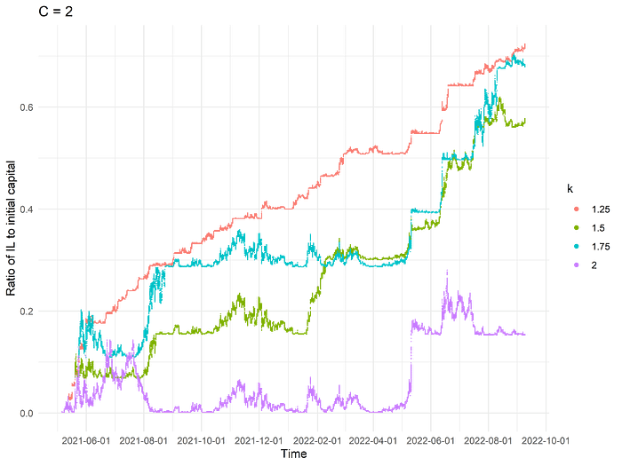
Perhaps surprisingly, at least in the case of C = 2, introducing this new parameter k only increases the realized IL. Visually, the patterns in the plot above suggest, as before, that we are subject to the same phenomenon where any rebalance away from the exact midpoint "locks in" the IL there, whereas a wider range allows matural mean reversion to reduce unrealized IL back to much lower levels.
To be a bit more systematic, we can test a wide range of values of both C and k. Specifically, we try the same range of C values as earlier and, each time, consider values of k equal to 20%, 40%, ..., 100% of the corresponding value of C:
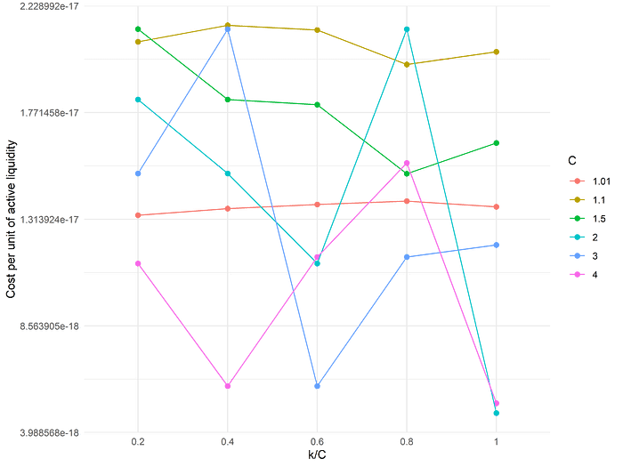
In general, the pattern that we observed holds: it is generally unproductive to add in the parameter k on top of our initial scenario, and optimal results are attained by setting C = 2 or C = 4 without the addition of k, as before. (For quite low values of C, such as C = 1.01 or C = 1.1, it does appear that lowering k improves the results slightly, but not to a degree such that they are competitive with simply setting C = 4 alone.) Ultimately, it appears that simply rebalancing "early" yields little benefit in and of itself.
One might then reasonably contest that a swap fee of zero is overly unrealistic. Even if there is no uninformed flow whatsoever and all swaps are arbitrages against an external market, those swaps still provide some fee accrual to liquidity providers (even if the value captured by the arbitrageur is substantially higher than the fee extracted). At the same time, this does change the simulation in other small ways; for example, assuming that rebalancing is done via direct swap execution rather than resting limit orders, each rebalance now also incurs a small fee.
While we did model the effects of adding in a fee, we felt the effects were quite marginal at any realistic fee tier and are not worth presenting in great detail. In general, the impact of modeling a swap fee was fairly independent of the specific parameterization of the rebalancing strategy, and in any case had little effect.
Finally, there is one last modification, perhaps more compelling than the others, that readily comes to mind. As we have seen so far, the basic reason why simple rebalancing strategies lose money is because they are in some sense excessively shorting the mean reversion of ETH prices. For example, if ETH prices go up enough that the liquidity position is no longer in range, the position rebalances to center around that new range, “locking in” impermanent losses; however, if the position had been slightly wider (enough so that the price of ETH always stayed in range), it appears to often be the case that ETH prices mean revert sufficiently such that impermanent losses decline to much lower levels and never get “locked in” by a rebalancing event.
This observation directly suggests that it might be beneficial to simply wait for ETH prices to mean-revert back into range! In particular, we can specify that a liquidity position only rebalances around a new ETH price if it has been out of range for more than H seconds. In principle, setting an appropriate value of H should allow us to partially account for the mean-reverting tendency of ETH prices, substantially ameliorating the tendency of rebalancing strategies to prematurely "lock in" impermanent losses yet allowing us to set a narrower range with a higher liquidity concentration factor.
For different values of C (position width), we tested values of H ranging from 0 (null value) to as long as 1 entire month. The results are plotted below, where each continuous colored line represents runs with different values of H, holding C (position width) constant:

Across all values tested, technically speaking, the minimum cost per active liquidity is attained with a range position width of C = 1.7 and a value of H equal to 168 hours (7 days), meaning that a liquidity position is allowed to stay out of range for 7 full days before it is rebalanced around the current price.
In general, when position range (C) is held fixed, increasing H qualitatively appears to make the cost per unit liquidity cheaper up to a certain point, after which it steadily grows increasingly expensive. This makes sense: there is generally some optimal value of H which is nonzero; however, when H is brought too large, even if impermanent losses stay low, the position is inactive for increasingly greater amounts of time, increasing the overall cost per unit of active liquidity supplied over the range of time studied. However, the variation in cost per unit liquidity induced by modulating H is ultimately far lower than the variation induced by modulating the position width, and the best parameter set very barely outperforms setting a width of C = 2 or C = 4 with no additional parameters whatsoever.
From a practical perspective, the impact of the parameter H is sufficiently minimal that it would be better to ignore it rather than to risk overfitting C and H jointly.
Conclusion
In the above analysis, we established a framework for testing different strategies for the purpose of automated liquidity management. Taking the perspective of a protocol or DEX which wants to determine the most cost-effective way to seed initial token liquidity, we set up a series of backtests with rebalancing strategies similar to those implemented by popular liquidity vault yield protocols.
Although our analysis is exceedingly simple, it does suggest that there is no “free lunch” here. That is not really so surprising; at the end of the day, simple automatic rebalancing strategies are likely too simple to model the price evolution of an asset like ETH.
Some of the popular liquidity vaults do go further; for example, Gamma claims to apply “machine learning” to predict future mean reversion, and Charm Finance has a more sophisticated dual-position strategy. We have experimented with these additional layers of complexity, with relatively modest results, which we hope to present in full in a future post.
In sum, the work we have done so far converges on a very simple recommendation for “seeding” asset liquidity: pick a very wide range and keep it simple. While our results only indirectly bear upon the profitability of liquidity vaults, we do feel that they present a somewhat bearish outlook for the fundamental ability for simple automated strategies to deliver high, or even positive, yields to depositors. That may be one reason, among others, why vaults seem to have slowly died off in popularity after an initial spike.
-0xfbifemboy